OSMnx is a Python package used for modeling ubran geographic features and relationships. Drawing on volunteer-supplied data at OpenstreetMap, OSMnx facilitates the geoanalytics of various aspects of urban life such as travel networks and accesibility, zoning or public health. OSMnx is a useful tool for urban planning. The global data that this API opens up is publicly accessible through the OpenstreetMap portal.
In this notebook we’ll go over some of the basic features of OSMnx.
Relevant Python Packages
For starters we’ll need to load the OSMnx package together with Matplotlib for visualization. Under the hood, OSMnx extends the Overpass package, wrapping it in a more elegant API. OSMnx also uses Geopandas, which in turn extends the Pandas library with geocoding features.
!pip install osmnx!pip install matplotlibimport osmnx as oximport matplotlibimport matplotlib.pyplot as pltprint(ox.__version__)print(matplotlib.__version__)
Requirement already satisfied: osmnx in /opt/conda/lib/python3.12/site-packages (2.0.5)
Requirement already satisfied: geopandas>=1.0.1 in /opt/conda/lib/python3.12/site-packages (from osmnx) (1.1.1)
Requirement already satisfied: networkx>=2.5 in /opt/conda/lib/python3.12/site-packages (from osmnx) (3.4.2)
Requirement already satisfied: numpy>=1.22 in /opt/conda/lib/python3.12/site-packages (from osmnx) (2.1.3)
Requirement already satisfied: pandas>=1.4 in /opt/conda/lib/python3.12/site-packages (from osmnx) (2.2.3)
Requirement already satisfied: requests>=2.27 in /opt/conda/lib/python3.12/site-packages (from osmnx) (2.32.3)
Requirement already satisfied: shapely>=2.0 in /opt/conda/lib/python3.12/site-packages (from osmnx) (2.1.1)
Requirement already satisfied: pyogrio>=0.7.2 in /opt/conda/lib/python3.12/site-packages (from geopandas>=1.0.1->osmnx) (0.11.0)
Requirement already satisfied: packaging in /opt/conda/lib/python3.12/site-packages (from geopandas>=1.0.1->osmnx) (24.2)
Requirement already satisfied: pyproj>=3.5.0 in /opt/conda/lib/python3.12/site-packages (from geopandas>=1.0.1->osmnx) (3.7.1)
Requirement already satisfied: python-dateutil>=2.8.2 in /opt/conda/lib/python3.12/site-packages (from pandas>=1.4->osmnx) (2.9.0.post0)
Requirement already satisfied: pytz>=2020.1 in /opt/conda/lib/python3.12/site-packages (from pandas>=1.4->osmnx) (2024.1)
Requirement already satisfied: tzdata>=2022.7 in /opt/conda/lib/python3.12/site-packages (from pandas>=1.4->osmnx) (2025.1)
Requirement already satisfied: charset_normalizer<4,>=2 in /opt/conda/lib/python3.12/site-packages (from requests>=2.27->osmnx) (3.4.1)
Requirement already satisfied: idna<4,>=2.5 in /opt/conda/lib/python3.12/site-packages (from requests>=2.27->osmnx) (3.10)
Requirement already satisfied: urllib3<3,>=1.21.1 in /opt/conda/lib/python3.12/site-packages (from requests>=2.27->osmnx) (2.3.0)
Requirement already satisfied: certifi>=2017.4.17 in /opt/conda/lib/python3.12/site-packages (from requests>=2.27->osmnx) (2025.1.31)
Requirement already satisfied: six>=1.5 in /opt/conda/lib/python3.12/site-packages (from python-dateutil>=2.8.2->pandas>=1.4->osmnx) (1.17.0)
Requirement already satisfied: matplotlib in /opt/conda/lib/python3.12/site-packages (3.10.1)
Requirement already satisfied: contourpy>=1.0.1 in /opt/conda/lib/python3.12/site-packages (from matplotlib) (1.3.1)
Requirement already satisfied: cycler>=0.10 in /opt/conda/lib/python3.12/site-packages (from matplotlib) (0.12.1)
Requirement already satisfied: fonttools>=4.22.0 in /opt/conda/lib/python3.12/site-packages (from matplotlib) (4.56.0)
Requirement already satisfied: kiwisolver>=1.3.1 in /opt/conda/lib/python3.12/site-packages (from matplotlib) (1.4.8)
Requirement already satisfied: numpy>=1.23 in /opt/conda/lib/python3.12/site-packages (from matplotlib) (2.1.3)
Requirement already satisfied: packaging>=20.0 in /opt/conda/lib/python3.12/site-packages (from matplotlib) (24.2)
Requirement already satisfied: pillow>=8 in /opt/conda/lib/python3.12/site-packages (from matplotlib) (11.1.0)
Requirement already satisfied: pyparsing>=2.3.1 in /opt/conda/lib/python3.12/site-packages (from matplotlib) (3.2.1)
Requirement already satisfied: python-dateutil>=2.7 in /opt/conda/lib/python3.12/site-packages (from matplotlib) (2.9.0.post0)
Requirement already satisfied: six>=1.5 in /opt/conda/lib/python3.12/site-packages (from python-dateutil>=2.7->matplotlib) (1.17.0)
2.0.5
3.10.1
OpenstreetMap Data Structures and Constructs
OSM abstracts geographic features as geometric primitives: points (nodes), lines (ways) and polygons (relations). Openstreetmap uses these primitives as the basis to encode urban constructs. For example, points locate urban entities such as cafes, museums or hospitals. Together they are conceptually known as points of interest (POI). As building blocks, an ordered set of points constitute lines that represent road connections. In turn these lines become the building blocks of polygons which stand for physical entities (buildings or parks) or virtual regions (towns, districts, etc.)
OSM assigns unique IDs to every primitive it tracks. Some OSMnx functions can lookup these primitives by their canonical name or by a string representation of their OSM ID. For entities that are nondescript – such as a corner of a park – we only have the OSM ID as a reference handle.
For example, as OSM sees it, Ueno may refer to a railway station in Tokyo, Japan; at the same time it also refers to the administrative boundary in the metropolis. The first entity is a node while the other is a relation. The OSM ID distinguishes between the two clearly (“N” as a node; “R” as a relation):
Ueno Station: “N8300320717”
Ueno Admin: “R18158684”
Acquiring Points of Interest (POI) Data
The geodataframe is the basic data structure of OSMnx. Organized as a tabular set of rows and columns, the GDF encodes urban data such as geometry, address, amenity categories, contact information (telephone, email or website) – information we deal with when we talk about places we live or work in, a destinations we travel to or a region worth noting. Essentially, working with OSMnx involves fetching geodataframes from Openstreetmap and manipulating the information in order to transform it in ways that are relevant to us, perhaps as a table, a map or as a data plot.
Let’s get the information for Minato, a city in Metopolitan Tokyo (not to be confused with Minato Ward in Nagoya). The city is outlined in orange in the screenshot above taken from Openstreetmap. The following code uses features_from_place() to query OSM. We supply the place we’re interested in – formally known as the OSM administrative boundary – along with a dictionary of tags to filter the information we want.
OSM tags are organized in a sets of keys and tags. In Python they are reprsented as a dictionary type. A handy reference for the top-level OSM keys are found here.
minato_poi = ox.features_from_place('Minato, Tokyo', tags={'amenity': ['cafe', 'pub'], 'tourism':['museum', 'hotel', 'attraction'], 'building':['office', 'retail']})print(f"{len(minato_poi)} elements in {type(minato_poi)}\n\n")print(minato_poi.columns)minato_poi.head(3)
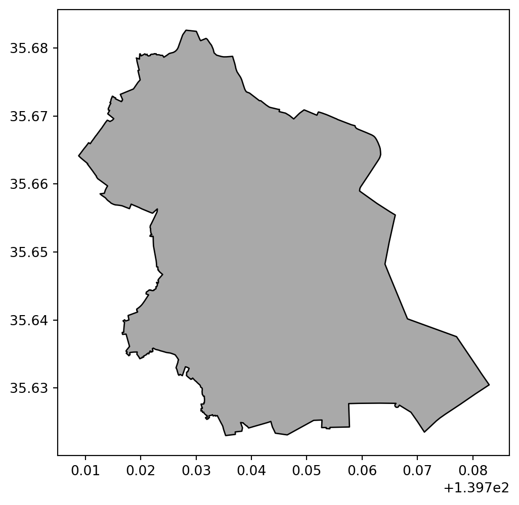
Can we query OSM for information and visualize it as a plot? Yes, we can. In the example below we turn to the geocode_to_gdf() to retrieve polygonal information suitable for plotting. Commented out, we also show the same function call using the OSM ID for Minato City: 1761717.
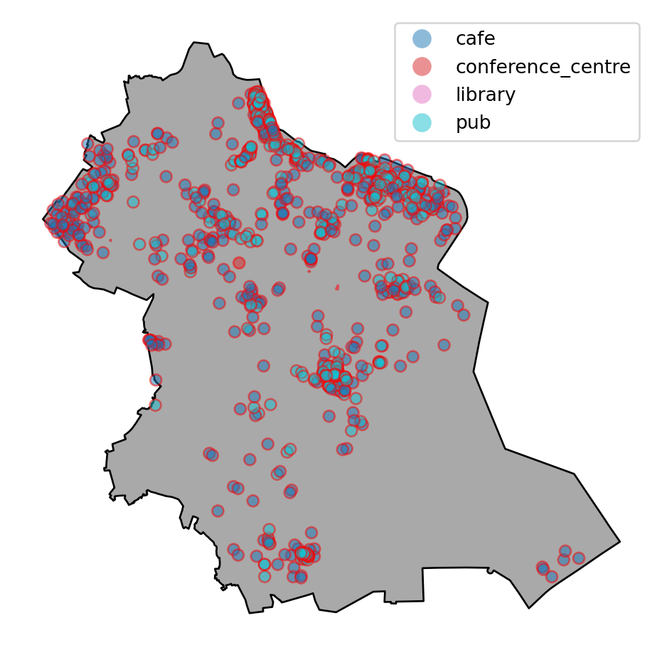
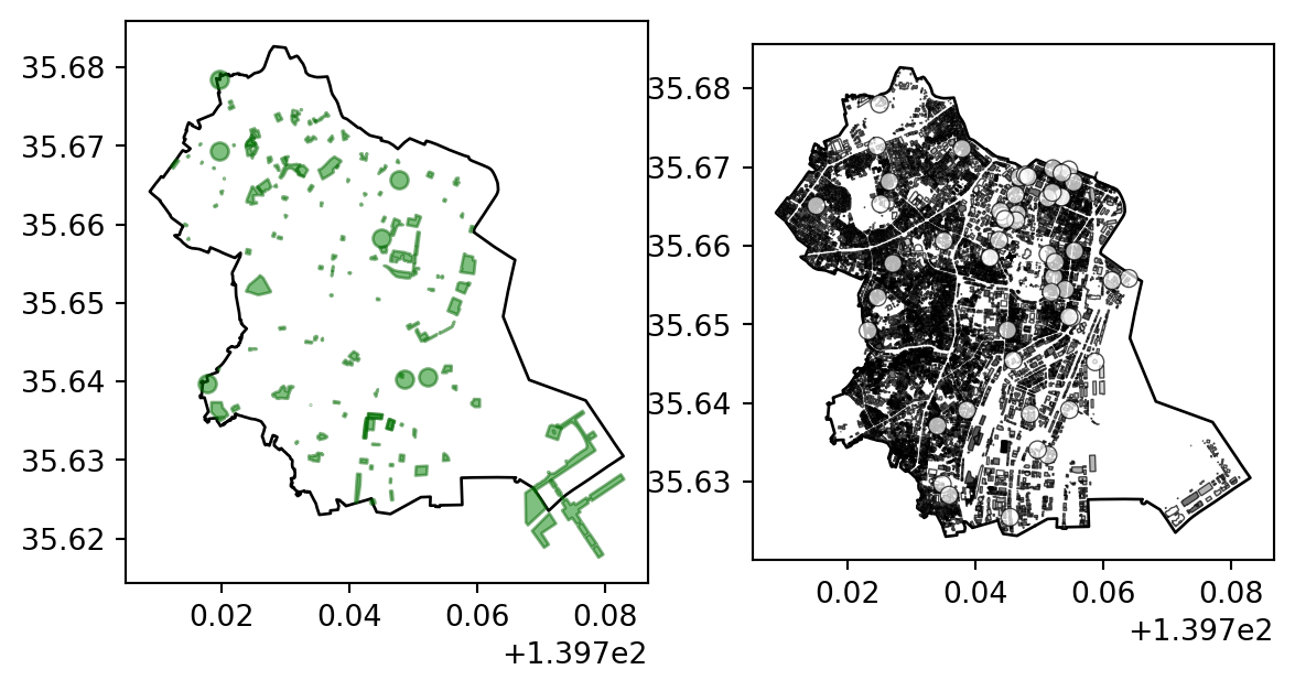
Using Matplotlib, we can combine information about Minato points of interest (POI) together with its polygonal representation into one infographic. In the example below, we make more than one plot() call to accomplish this. Note that we plot POIs by selecting a column-key of the GeoDataFrame, in this case amenity.
# Create a plot to visualize the admin boundary and POIsf, ax = plt.subplots(1, 1, figsize=(6,6))# Plot the administrative boundaryadmin_minato.plot(ax=ax, color='darkgrey', edgecolor='k')# Plot the amenity POIminato_poi.plot(column='amenity', ax=ax, alpha=0.5, edgecolor='red', legend=True)# Customize the plotax.axis('off')plt.show()
Acquiring Polygonal Data
While plotting points of intererest is useful, the information doesn’t convey the geographic scope of particular urban features such as buildings, for example. These are urban entities better visualized as polygons.
Let’s begin by re-querying OSM about the Minato administration boundary. Then let’s focus on a subset of GeoDataFrame, the polygons for this administrative region. Finally, with the polygonal data in hand, let’s filter the information according to the same tags we’ve used before.
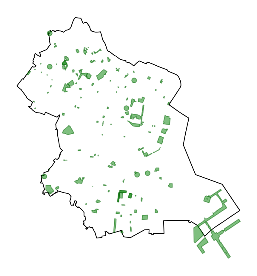
OK, as we’ve done earlier for the POIs, let’s overlay plots for the two polygonal data sets we’ve gathered.
# Create a plot to visualize the admin boundary and park polygonsf, ax = plt.subplots(1, 1, figsize=(6, 6))# Plot the Minato administrative boundaryminato_district.plot(ax=ax, color='none', edgecolor='k')# Plot the parks in Minato Cityminato_parks.plot(ax=ax, color='green', alpha=0.5, edgecolor='darkgreen')# Customize the plotax.axis('off')plt.show()
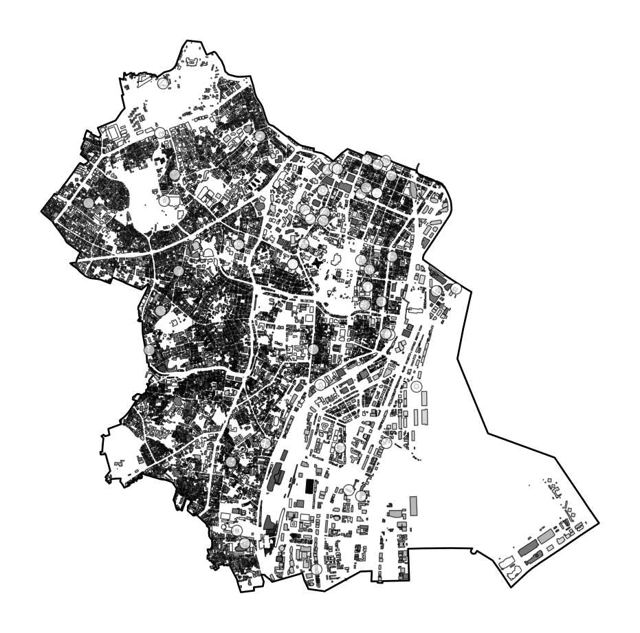
Now that we’ve looked at the park amenities at Minato City, let’s inspect all the building features regardless of subtype and pass it onto Matplotlib.
minato_buildings = ox.features_from_polygon(minato_polygon, tags={'building': True})print(f"{len(minato_buildings)} elements in {type(minato_buildings)}\n\n")minato_buildings.columns
26175 elements in <class 'geopandas.geodataframe.GeoDataFrame'>
f, ax = plt.subplots(1, 1, figsize=(6, 6))# Plot the Minato administrative boundaryminato_district.plot(ax=ax, color='none', edgecolor='k')# Plot the parks in Minato Cityminato_buildings.plot(ax=ax, cmap ='Greys', edgecolor ='black', alpha =0.7, linewidth =0.5)# Customize the plotax.axis('off')plt.show()
With a little variation to the Matplotlib function calls, we can visualize the parks and buildings maps together.
f, ax = plt.subplots(1, 2, figsize=(7, 4))# Plot the Minato administrative boundaryminato_district.plot(ax=ax[0], color='none', edgecolor='k')# Plot the parks in Minato Cityminato_parks.plot(ax=ax[0], color='green', alpha=0.5, edgecolor='darkgreen')# Plot the Minato administrative boundaryminato_district.plot(ax=ax[1], color='none', edgecolor='k')# Plot the parks in Minato Cityminato_buildings.plot(ax=ax[1], cmap ='Greys', edgecolor ='black', alpha =0.7, linewidth =0.5)plt.show()
Acquiring Graph Data
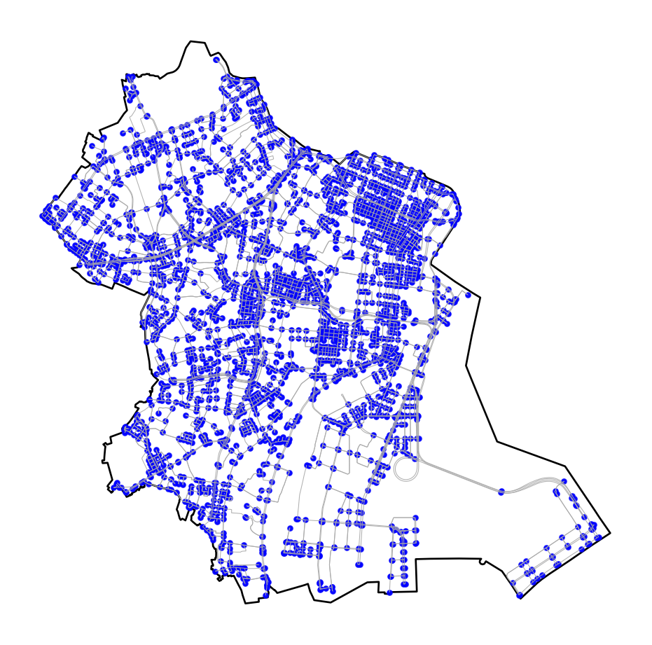
Urban analytics wouldn’t be complete without road networks. In OSM, that information is embedded in GDFs as graphs where a line represents a path and a node represents an intersection. OSM graphs are multi-directed graphs: a node is connected with roadways that are inbound or outbound (directed); several paths converge on a node junction (multi connected).
Let’s see how we can retrieve the graph data for Minato City.
The sequence of OSMnx operations are: * Retrieve GeoDataFrame data from OSM * Extract the polygonal data from the GDF * Given the set polygons, retrieve the graph network from OSM
# Download the road network for all transport modesminato_roads = ox.graph_from_polygon(minato_polygon, network_type='drive')print("Type of the road network graph (all modes):", type(minato_roads))print("Number of nodes (all modes):", minato_roads.number_of_nodes())print("Number of edges (all modes):", minato_roads.number_of_edges())
Type of the road network graph (all modes): <class 'networkx.classes.multidigraph.MultiDiGraph'>
Number of nodes (all modes): 2971
Number of edges (all modes): 6624
At this point our goal is to display the road network as a map bounded by the Minato City administrative region. To get there, we first need to transform the graph data into another GeoDataFrame.
# Convert the network graph to GeoDataFrames for nodes and edgesnodes, edges = ox.graph_to_gdfs(minato_roads)# Display the first few rows of the nodes GeoDataFramedisplay(nodes.head(3))# Display the first few rows of the edges GeoDataFramedisplay(edges.head(3))# Print the features stored in each GeoDataFrameprint("Keys in the nodes table:", list(nodes.keys()))print("Keys in the edges table:", list(edges.keys()))print()# Print the total number of nodes and edgesprint("Number of nodes in the node table:", len(nodes))print("Number of edges in the node table:", len(edges))
y
x
highway
ref
street_count
junction
geometry
osmid
31236584
35.634935
139.768683
motorway_junction
1101
3
NaN
POINT (139.76868 35.63494)
31236646
35.634417
139.777989
NaN
NaN
3
NaN
POINT (139.77799 35.63442)
31236657
35.633476
139.778439
NaN
NaN
3
NaN
POINT (139.77844 35.63348)
osmid
bridge
highway
lanes
oneway
reversed
length
geometry
name
ref
maxspeed
access
tunnel
width
junction
u
v
key
31236584
31236646
0
[4848889, 4848756, 820214407]
yes
motorway_link
1
True
False
971.162374
LINESTRING (139.76868 35.63494, 139.76895 35.6...
NaN
NaN
NaN
NaN
NaN
NaN
NaN
31236646
573342136
0
333682057
yes
tertiary
NaN
True
False
40.061292
LINESTRING (139.77799 35.63442, 139.77824 35.6...
NaN
NaN
NaN
NaN
NaN
NaN
NaN
31236657
298984113
0
863283179
yes
tertiary
NaN
True
False
101.078790
LINESTRING (139.77844 35.63348, 139.77788 35.6...
NaN
NaN
NaN
NaN
NaN
NaN
NaN
Keys in the nodes table: ['y', 'x', 'highway', 'ref', 'street_count', 'junction', 'geometry']
Keys in the edges table: ['osmid', 'bridge', 'highway', 'lanes', 'oneway', 'reversed', 'length', 'geometry', 'name', 'ref', 'maxspeed', 'access', 'tunnel', 'width', 'junction']

Number of nodes in the node table: 2971
Number of edges in the node table: 6624
No we can take this GDF and visualize it.
f, ax = plt.subplots(1,1,figsize=(6,6))# Plot the Minato administrative boundaryminato_district.plot(ax=ax, color='none', edgecolor='k')nodes.plot(ax=ax, color ='blue', markersize =5, alpha =0.9)edges.plot(ax=ax, color ='darkgrey', linewidth =0.4, alpha =0.9)ax.axis('off')
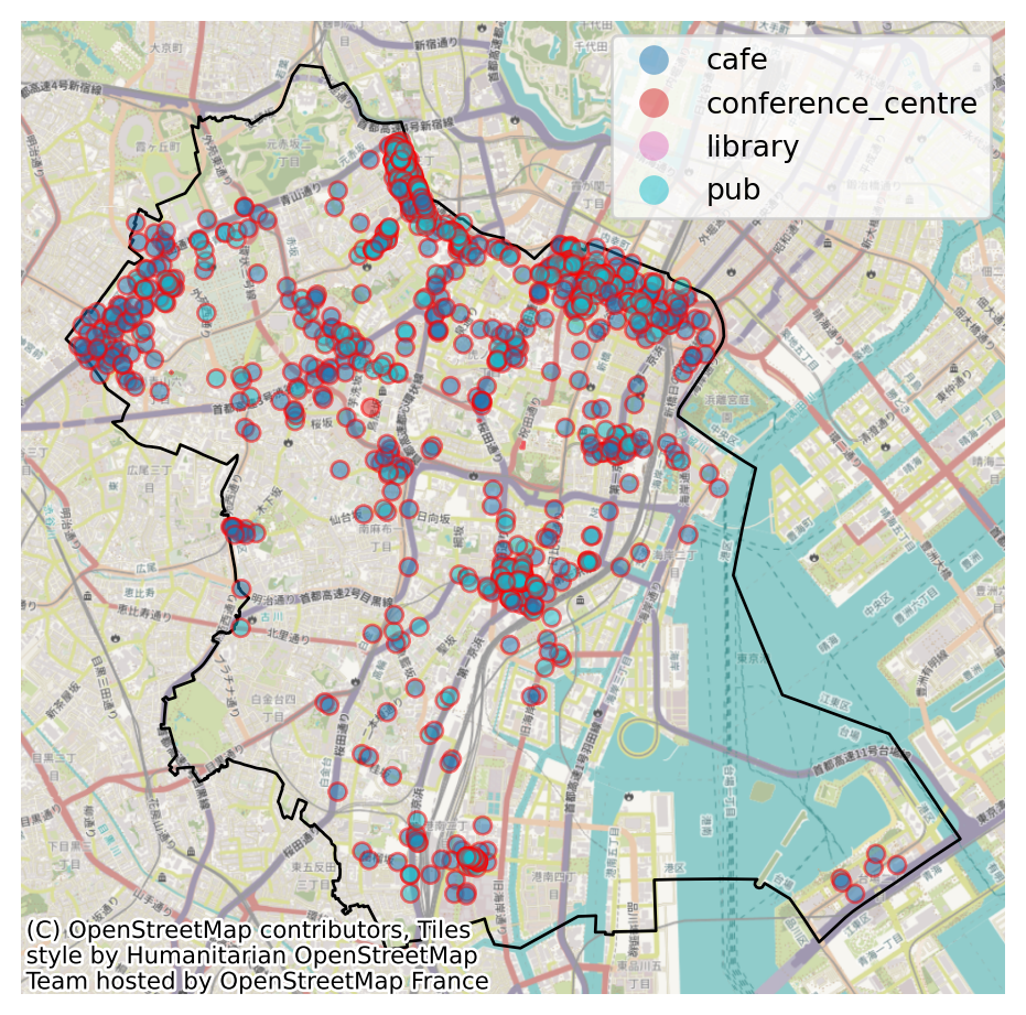
In the introductory section we showed a screen shot of Minato City taken directly from the Openstreetmap site. We can also achieve something like that with OSMnx combined with the Contextily package, overlaying OSM geometries over a map image in the background.
The Contextily site describes itself as a package to retrieve tile maps from the internet. In the background, the Contextily API queries a number of tile map providers, such as ESRI or CartoDB. For our purposes, we’ll re-render on of our Minato POI map (cafe, library, etc.) with a basemap provided by Contextily.
!pip install contextilyimport contextily as ctxprint(ctx.__version__)
Requirement already satisfied: contextily in /opt/conda/lib/python3.12/site-packages (1.6.2)
Requirement already satisfied: geopy in /opt/conda/lib/python3.12/site-packages (from contextily) (2.4.1)
Requirement already satisfied: matplotlib in /opt/conda/lib/python3.12/site-packages (from contextily) (3.10.1)
Requirement already satisfied: mercantile in /opt/conda/lib/python3.12/site-packages (from contextily) (1.2.1)
Requirement already satisfied: pillow in /opt/conda/lib/python3.12/site-packages (from contextily) (11.1.0)
Requirement already satisfied: rasterio in /opt/conda/lib/python3.12/site-packages (from contextily) (1.4.3)
Requirement already satisfied: requests in /opt/conda/lib/python3.12/site-packages (from contextily) (2.32.3)
Requirement already satisfied: joblib in /opt/conda/lib/python3.12/site-packages (from contextily) (1.4.2)
Requirement already satisfied: xyzservices in /opt/conda/lib/python3.12/site-packages (from contextily) (2025.1.0)
Requirement already satisfied: geographiclib<3,>=1.52 in /opt/conda/lib/python3.12/site-packages (from geopy->contextily) (2.0)
Requirement already satisfied: contourpy>=1.0.1 in /opt/conda/lib/python3.12/site-packages (from matplotlib->contextily) (1.3.1)
Requirement already satisfied: cycler>=0.10 in /opt/conda/lib/python3.12/site-packages (from matplotlib->contextily) (0.12.1)
Requirement already satisfied: fonttools>=4.22.0 in /opt/conda/lib/python3.12/site-packages (from matplotlib->contextily) (4.56.0)
Requirement already satisfied: kiwisolver>=1.3.1 in /opt/conda/lib/python3.12/site-packages (from matplotlib->contextily) (1.4.8)
Requirement already satisfied: numpy>=1.23 in /opt/conda/lib/python3.12/site-packages (from matplotlib->contextily) (2.1.3)
Requirement already satisfied: packaging>=20.0 in /opt/conda/lib/python3.12/site-packages (from matplotlib->contextily) (24.2)
Requirement already satisfied: pyparsing>=2.3.1 in /opt/conda/lib/python3.12/site-packages (from matplotlib->contextily) (3.2.1)
Requirement already satisfied: python-dateutil>=2.7 in /opt/conda/lib/python3.12/site-packages (from matplotlib->contextily) (2.9.0.post0)
Requirement already satisfied: click>=3.0 in /opt/conda/lib/python3.12/site-packages (from mercantile->contextily) (8.1.8)
Requirement already satisfied: affine in /opt/conda/lib/python3.12/site-packages (from rasterio->contextily) (2.4.0)
Requirement already satisfied: attrs in /opt/conda/lib/python3.12/site-packages (from rasterio->contextily) (25.3.0)
Requirement already satisfied: certifi in /opt/conda/lib/python3.12/site-packages (from rasterio->contextily) (2025.1.31)
Requirement already satisfied: cligj>=0.5 in /opt/conda/lib/python3.12/site-packages (from rasterio->contextily) (0.7.2)
Requirement already satisfied: click-plugins in /opt/conda/lib/python3.12/site-packages (from rasterio->contextily) (1.1.1.2)
Requirement already satisfied: charset_normalizer<4,>=2 in /opt/conda/lib/python3.12/site-packages (from requests->contextily) (3.4.1)
Requirement already satisfied: idna<4,>=2.5 in /opt/conda/lib/python3.12/site-packages (from requests->contextily) (3.10)
Requirement already satisfied: urllib3<3,>=1.21.1 in /opt/conda/lib/python3.12/site-packages (from requests->contextily) (2.3.0)
Requirement already satisfied: six>=1.5 in /opt/conda/lib/python3.12/site-packages (from python-dateutil>=2.7->matplotlib->contextily) (1.17.0)
1.6.2
# Create a plot to visualize the admin boundary and points of interestf, ax = plt.subplots(1, 1, figsize=(6,6))# Plot the administrative boundaryadmin_minato.plot(ax=ax, color='None', edgecolor='k')# Plot the amenity POIminato_poi.plot(column='amenity', ax=ax, alpha=0.5, edgecolor='red', legend=True)# Query ESRI to add basemap using Contextilyctx.add_basemap(ax, crs = admin_minato.crs, url=ctx.providers.Esri.WorldTopoMap)# Customize the plotax.axis('off')plt.show()