Pandas Basic Analysis 01: Intro

Python

Pandas

Jupyter

Data Analytics

Part one of data analysis with Python Pandas: introduction.

Author

Dennis Chua

Published

May 18, 2025

01 Basic Data Analysis with Python Pandas

Content Outline

Introduction
Load data from a text file
Display summary information about the data
Data analysis using the groupby() operation
Display data plots
Filtering data rows using the loc() method

Jupyter notebook

Data from Gapminder Foundation

Introduction

Pandas is a Python package used extensively in data manipulation and analysis. The purpose of this Colab notebook is to give an overview of Pandas. Subsequent notebooks in this tutorial series elaborate on various aspects of Pandas.

import pandas as pd

import matplotlib
import matplotlib.pyplot as plt

Load Data From a Text File

For this demonstration, we’ll work with global demographic data sourced from the Gapminder Foundation. Before proceeding, we load the tab-delimeted data file “gapminder.tsv” to Google Colab. The data is available from this Github repo.

df = pd.read_csv("sample_data/gapminder.tsv", sep='\t')

Display Summary Information About the Data

A cursory look at the data shows that it has six columns and 1704 rows. In Pandas, a set of row and columnar data is known as a data frame. Every data frame comes with an info() method that breaks down the tabulated data. The keys() method of a data frame returns a list of indices, or column names. To enumerate the column data themselves, a data frame’s values attribute returns the information as a two-dimensional array.

df.info()

<class 'pandas.core.frame.DataFrame'>
RangeIndex: 1704 entries, 0 to 1703
Data columns (total 6 columns):
 #   Column     Non-Null Count  Dtype  
---  ------     --------------  -----  
 0   country    1704 non-null   object 
 1   continent  1704 non-null   object 
 2   year       1704 non-null   int64  
 3   lifeExp    1704 non-null   float64
 4   pop        1704 non-null   int64  
 5   gdpPercap  1704 non-null   float64
dtypes: float64(2), int64(2), object(2)
memory usage: 80.0+ KB

df.keys()

Index(['country', 'continent', 'year', 'lifeExp', 'pop', 'gdpPercap'], dtype='object')

df.values

array([['Afghanistan', 'Asia', 1952, 28.801, 8425333, 779.4453145],
       ['Afghanistan', 'Asia', 1957, 30.332, 9240934, 820.8530296],
       ['Afghanistan', 'Asia', 1962, 31.997, 10267083, 853.10071],
       ...,
       ['Zimbabwe', 'Africa', 1997, 46.809, 11404948, 792.4499603],
       ['Zimbabwe', 'Africa', 2002, 39.989, 11926563, 672.0386227],
       ['Zimbabwe', 'Africa', 2007, 43.487, 12311143, 469.7092981]],
      dtype=object)

That was the structure of the data frame. Now let’s analayze the data itself. The Pandas describe() method reports the standard statistics for the data frame.

df.describe()

	year	lifeExp	pop	gdpPercap
count	1704.00000	1704.000000	1.704000e+03	1704.000000
mean	1979.50000	59.474439	2.960121e+07	7215.327081
std	17.26533	12.917107	1.061579e+08	9857.454543
min	1952.00000	23.599000	6.001100e+04	241.165876
25%	1965.75000	48.198000	2.793664e+06	1202.060309
50%	1979.50000	60.712500	7.023596e+06	3531.846988
75%	1993.25000	70.845500	1.958522e+07	9325.462346
max	2007.00000	82.603000	1.318683e+09	113523.132900

Data Analysis Using the Groupby() Operation

Let’s go deeper. Say we want to find the average life expectancy by year. Here’s how we instruct Pandas to retrieve that information.

df.groupby('year')['lifeExp'].mean()

year
1952    49.057620
1957    51.507401
1962    53.609249
1967    55.678290
1972    57.647386
1977    59.570157
1982    61.533197
1987    63.212613
1992    64.160338
1997    65.014676
2002    65.694923
2007    67.007423
Name: lifeExp, dtype: float64

One way of understanding what just happened is that Pandas separates and analzyes the data as buckets, each one representing a year. Judging by the result above, not all years are present in our data as we only see twelve non-contiguous years between 1952 and 2007.

Display Data Plots

Next we plot the graph for this data. Note that if we were to do so in the Python or iPython interactive console, we’d have to first import a Python display library, Qt for example, for displaying the graph as a GUI window; then we register it to matplotlib just before we run the show() method: * import PyQt5 * matplotlib.use(‘Qt5Agg’)

df.groupby('year')['lifeExp'].mean().plot()
plt.show()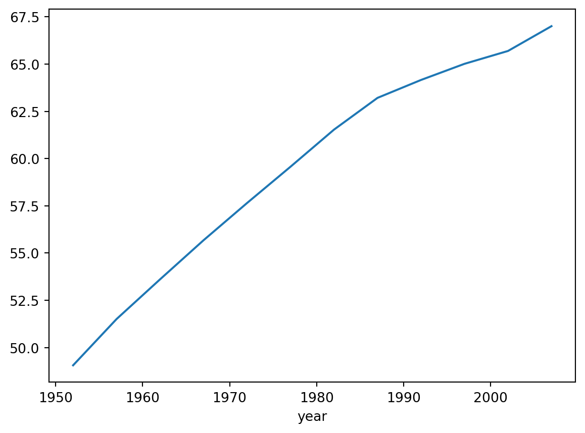

Now let’s go a bit further. Say we want to find the life expentancy data grouped by year and by country.

df.groupby(['year', 'country'])[['pop', 'lifeExp']].mean()

		pop	lifeExp
year	country
1952	Afghanistan	8425333.0	28.801
	Albania	1282697.0	55.230
	Algeria	9279525.0	43.077
	Angola	4232095.0	30.015
	Argentina	17876956.0	62.485
...	...	...	...
2007	Vietnam	85262356.0	74.249
	West Bank and Gaza	4018332.0	73.422
	Yemen, Rep.	22211743.0	62.698
	Zambia	11746035.0	42.384
	Zimbabwe	12311143.0	43.487

1704 rows × 2 columns

Filtering Data Rows Using the loc() Method

This is a lot of information to take in and Pandas only presents a snapshot of the 1704 rows. To make it easier for ourselves, we can ask Pandas to limit the information to a list of years, say 1972, 1982 qne 1987. We use Panda’s loc() method to filter rows based on their label.

df.groupby(['year', 'country'])[['pop', 'lifeExp']].mean().loc[[1972, 1982, 1987]]

		pop	lifeExp
year	country
1972	Afghanistan	13079460.0	36.088
	Albania	2263554.0	67.690
	Algeria	14760787.0	54.518
	Angola	5894858.0	37.928
	Argentina	24779799.0	67.065
...	...	...	...
1987	Vietnam	62826491.0	62.820
	West Bank and Gaza	1691210.0	67.046
	Yemen, Rep.	11219340.0	52.922
	Zambia	7272406.0	50.821
	Zimbabwe	9216418.0	62.351

426 rows × 2 columns

It’s worth discussing a few fine points about Panda’s concept of a data row. Before we grouped the data by year, a row was a unit of information in the gapminder.tsv data file. That is, the original Pandas data frame was made up of all 1704 rows. However, now that we applied the groupby() method, Pandas organized the data such that a row bundles information by year. In this new, derived data frame, a row is now indexed by the year: 1972, 1982 and so on. Therefore when we apply the loc() method, we’re filtering these subset of grouped-by rows, not the original rows in the data file.

Applying the loc() method a number of times, we can futher refine the rows of information we extract for a particular year.

df.groupby(['year', 'country'])[['pop', 'lifeExp']].mean().loc[1972].loc[['Albania', 'Brazil', 'Vietnam']]

	pop	lifeExp
country
Albania	2263554.0	67.690
Brazil	100840058.0	59.504
Vietnam	44655014.0	50.254